
Buiding a 3D perception stack - Part 0
When we talk about an autonomous vehicle or any robot navigating its environment, perception fundamentally is about understanding the 3D space around it. For a self-driving car, this boils down to identifying what areas are drivable or navigable, and which are not. We need to build an instantaneous 3D understanding of the world relative to our own vehicle – the “ego” vehicle. Automotive computer vision stacks typically use machine learning (ML) based techniques to identify objects of interest, understand behavioral intent, and track dynamic objects in the scene.
My background has largely been in building deep learning-based computer vision stacks for automotive applications, often involving monocular depth estimators, detectors, and semantic segmentation. Advancements in hardware have enabled tight coupling between these ML models with 3D perception pipelines. Some perception stacks also use end-to-end pipelines, directly ingesting sensor data and predicting path trajectories. However, power and compute constrained applications (like drones and robots) still favor tight coupling of lightweight ML pipelines and 3D perception stacks – Traditional methods, like stereo vision, become particularly interesting.
In the past few months, I’ve been interested in understanding the limits of perception using low cost sensors such as cameras and IMUs. In this part, I set up visualization, a dataset and demonstrate a quick stereo vision pipeline; Finally, I set up the problem space for further exploration.
A simple Stereo Vision pipeline
Just like how humans interpret the depth of a scene using our two eyes, a stereo camera setup can help us recover depth. By capturing two images from slightly different viewpoints, we can use feature matching and triangulation to figure out how far away objects are. Let’s calculate the depth of the scene using a stereo setup.
To get started, we’re using the Argoverse 2 self-driving dataset, which provides 15-second sequences of synchronized data, including a forward-facing stereo camera pair, 7 ring cameras, 2 roof mounted lidars, along with localization data in world coordinates. More details on the dataset available here.
For visualizing and debugging our perception pipeline, I’ve been exploring a new tool called Rerun. It offers Rust and Python APIs, letting us log various types of information—images, poses, and point clouds—along with their respective timesteps. This creates a navigable timeline, which is incredibly useful for debugging. The UI has a familiar feel, similar to Foxglove, but unlike Foxglove, Rerun is designed to run entirely on the client side, though both leverage websockets for observing headless systems.
Loading Argoverse 2 and using Rerun
Let’s first start loading data from disk using the Argoverse 2 (av2) API. av2 has limited API documentation but, after reading through the codebase, seems to provide intuitive abstraction across concepts used in the perception space (Intrinsics, Pinhole, SE3). By parsing the provided examples, I was able to use SensorDataloader to access synchronized camera and lidar data. Each synchronized datum contains the timestamp, image data (if available), and the corresponding intrinsics and extrinsics. Below a rough tree of how the relationships of the components map out within the API:
SensorDataloader
│
├──    Sweep                            # LiDAR sweep
├──    TimestampedCitySE3EgoPoses       # mapped against timestamp_ns
│      └── SE3                          # contains R and T
├──    int timestamp_ns
├──    CuboidList                       # Annotations
└──    Dict[str, TimestampedImage]]
            │    ├── NDArray img
            │    ├── PinholeCamera
            │    │   ├── SE3 ego_SE3_cam
            │    │   ├── Intrinsics
            │    │   └── "cam_name"
            │    └── int timestamp_ns
            └── "cam_name"
Now, let’s start logging this information into Rerun, specifically the stereo left and right images. Before we start logging, we have the choice to set up the structure of the viewer. Layouts in Rerun are defined using blueprints similar to the one below:
import rerun.blueprint as rrb

sensor_views = [rrb.Spatial2DView(
                name=StereoCameras.STEREO_FRONT_LEFT,
                origin=f"world/ego_vehicle/{StereoCameras.STEREO_FRONT_LEFT}"
                ),
                rrb.Spatial2DView(
                name=StereoCameras.STEREO_FRONT_RIGHT,
                origin=f"world/ego_vehicle/{StereoCameras.STEREO_FRONT_RIGHT}"
                ),
                rrb.Spatial2DView(
                name="stereo_disparity",
                origin="world/ego_vehicle/stereo_disparity"
                ),
                rrb.Spatial2DView(
                name="stereo_depth",
                origin=f"world/ego_vehicle/stereo_depth"
                )]

# Set up blueprint
blueprint = rrb.Vertical(
    rrb.Spatial3DView(name="3D", origin="world"),
    rrb.Grid(*sensor_views),
    row_shares=[4, 2],
)

rr.send_blueprint(blueprint=blueprint)
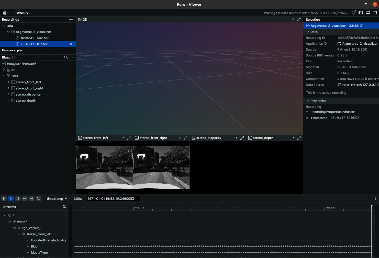
The simple blueprint results in the UI shown above. As we iterate through the dataset, we can log and view these images in Rerun.
Stereo Vision
Now that we have Rerun capturing data, let’s use OpenCV to calculate depth from the stereo setup. The fundamental problem we are trying to solve is one of correspondences between the left and right image – closer objects will have a larger shift relative to distant objects. To find correspondences between the left and right images, we employ a Semi-Global Block Matcher (SGBM). SGBM calculates a per-pixel matching cost over a small block and then aggregates these costs along multiple 1D paths – typically in eight directions; regular block matches find correspondences only along a single 1D path. The “semi-global” approach offers improved sub-pixel accuracy and creates more coherent surfaces. However, it does come at the cost of being slower and consuming more memory than basic block matching. We can fine-tune its performance by adjusting parameters like blockSize, numDisparities, and smoothness weights to balance noise reduction and edge preservation.
The images in the Argoverse dataset have already been rectified and undistorted which means we can directly use the provided camera intrinsics and extrinsics to extract depth.
Note: If the camera were to have dissimilar focal lengths or rectangular pixels (uncommon), you would have to run through cv2.stereoRectify() to the projection matrices to each view from which you can extract the focal length and baseline required to convert to depth.
# Example to get f and baseline when using dissimilar
# focal lengths/non-square pix
def get_stereo_calib_data(left_cam_obj, right_cam_obj):
    egoveh_se3_left = left_cam_obj.ego_SE3_cam
    egoveh_se3_right = right_cam_obj.ego_SE3_cam
    right_se3_egoveh = egoveh_se3_right.inverse()
    right_se3_left = right_se3_egoveh.compose(egoveh_se3_left).transform_matrix

    R = right_se3_left[:3, :3]
    T = right_se3_left[:3, 3]

    left_intrinsics = left_cam_obj.intrinsics.K
    right_intrinsics = right_cam_obj.intrinsics.K

    R1, R2, P1, P2, Q, roi1, roi2 = cv2.stereoRectify(
                                    left_intrinsics,
                                    np.array([0,0,0,0,0]),
                                    right_intrinsics,
                                    np.array([0,0,0,0,0]),
                                    (left_cam_obj.width_px,
                                        left_cam_obj.height_px),
                                    R=R,
                                    T=T,
                                    flags=cv2.CALIB_ZERO_DISPARITY,
                                    alpha=0)

    f = P1[0,0]
    baseline = P2[0,3]/-f

    return f, baseline
I’m planning to run the algorithm at 1/4th resolution of the captured data; The code snippet defines an appropriate SGBM matcher for the task. Using the f and baseline values we calculated previously, we can get the depth of the scene from the disparity!
def compute_disparity_sgbm(left, right, focal_length, baseline,
                          min_disp=0,
                          num_disp=16*8,
                          block_size=5,
                          raw=False):
    """
    Compute a disparity map from rectified stereo pair using SGBM.

    Parameters:
    - left, right: Grayscale uint8 rectified images.
    - min_disp: Minimum possible disparity value.
    - num_disp: Maximum disparity minus min_disp. Must be divisible by 16.
    - block_size: Matched block size. Must be odd (typically 3..11).

    Returns:
    - disp8: uint8 disparity map normalized to [0,255].
    """
    # SGBM parameters
    matcher = cv2.StereoSGBM_create(
        minDisparity=min_disp,
        numDisparities=num_disp,
        blockSize=block_size,
        P1=8 * 3 * block_size**2,
        P2=32 * 3 * block_size**2,
        disp12MaxDiff=1,
        preFilterCap=63,
        uniquenessRatio=10,
        speckleWindowSize=100,
        speckleRange=32,
        mode=cv2.STEREO_SGBM_MODE_SGBM_3WAY
    )

    # Compute disparity and convert from fixed‐point (×16) to float
    disp = matcher.compute(left, right)  #.astype(np.float32) / 16.0

    disp, _ = cv2.filterSpeckles(disp, 0, 60, num_disp)
    disp = disp.astype(np.float32) / 16.0

    # z = baseline * focal_length / disparity
    valid = disp > 0
    depth = np.zeros_like(disp, dtype=np.float32)
    depth[valid] = baseline * focal_length / disp[valid]

    if raw:
        return disp, depth
    # Normalize to 0..255 and convert to uint8 for display
    disp8 = normalize_for_display(disp)
    depth8 = normalize_for_display(depth)

    return disp8, depth8
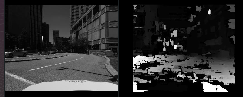
Before we publish our point clouds, let’s dissect this disparity map. By definition, we expect to have higher disparities for objects closer to us than those further out. While we do a gradient across relative distances, there are some significant errors. This is because stereo matching or matching in general is still fundamentally a hard correspondence problem which results in speckles and holes in the scene. Textureless surfaces like the hood of the car and regions in the sky are significantly affected. Errors might also be introduced also in regions with repetitive patterns and occlusions. Additionally, we are relaxing many conditions that the creators of the Argoverse dataset have address (brightness consistency, rolling vs global shutter, synchronization issues).
Regardless, let’s inverse project our points to 3D. Making sure to use the scaled intrinsics, we can project to 3D using the depth information obtained in the previous step. Let’s also record the intensity of the corresponding pixels to add colors to the points.
def project_to_3D(depth, cam_data, img=None):
    """ Project pixels to 3D """
    point_data = {}
    scaled_obj = cam_data.camera_model.scale(SCALE)
    K = scaled_obj.intrinsics.K
    K_inv = np.linalg.inv(K)

    H, W = depth.shape

    # 1) Create a grid of (u, v) pixel coordinates
    u = np.arange(W)
    v = np.arange(H)
    uu, vv = np.meshgrid(u, v)

    # 2) Stack to shape (3, H*W): [u; v; 1]
    ones = np.ones_like(uu)
    pix_homog = np.stack([uu, vv, ones], axis=0).reshape(3, -1)  # (3, N)

    # 3) Directions in camera space: (3,3) @ (3,N) → (3,N)
    dirs = K_inv @ pix_homog

    # 4) Scale each direction by its depth
    depth_flat = depth.reshape(1, -1)                  # (1, N)
    points_cam = dirs * depth_flat                    # (3, N)

    # 5) Transpose to (N,3) point list
    point_data["points"] = points_cam.T

    if img is not None:
        # colors expects an rgb img
        rgb = np.dstack((img, img, img))          # (H, W, 3)

        # now flatten it to a list of N = H*W colors
        colors = rgb.reshape(-1, 3)               # (N, 3)

        point_data["colors"] = colors
    else:
        point_data["colors"] = None

    return point_data
To publish this cloud to rerun, we use the Points3D component. Additionally, I want to record the motion of the vehicle across the scene. The argoverse dataset provides localization information in the city coordinate frame in the form of SE(3) rigid body transforms. If one uses the av2 API to load the data, the poses are available as an SE3 object which support compose() and invert() operations. Since the goal was to visualize a single scene, let’s consider the initial pose to be our origin. We can then transform subsequent poses and log relative motion to Rerun using the Transform3D component.
if world_se3_initpose == 0:
    # Initialize origin point
    world_se3_initpose = datum.timestamp_city_SE3_ego_dict[datum.timestamp_ns]

# Start from origin
world_se3_currentpose = datum.timestamp_city_SE3_ego_dict[datum.timestamp_ns]
initpose_se3_currentpose = world_se3_initpose.inverse().compose(world_se3_currentpose)
.
.
.
.
# Get 3D points
points_data = project_to_3D(depth, left_data,
                            img=downsize(left_data.img, fx=SCALE, fy=SCALE))
# Obtaining axis angle for rerun
axis, _ = cv2.Rodrigues(R_fixed)
angle = np.linalg.norm(axis)

# log 3D ego position in time
rr.log(
    f"/world/ego_vehicle",
    rr.Transform3D(
        translation=T_fixed,
        rotation=rr.RotationAxisAngle(axis=axis, angle=angle),
        relation=rr.TransformRelation.ChildFromParent)
    )
# log pinhole model
rr.log(
    f"world/ego_vehicle/{StereoCameras.STEREO_FRONT_LEFT}",
    rr.Pinhole(
        resolution=[left_cam.width_px, left_cam.height_px],
        focal_length=[left_cam.intrinsics.fx_px, left_cam.intrinsics.fy_px],
        principal_point=[left_cam.intrinsics.cx_px, left_cam.intrinsics.cy_px])
    )

# Display 3D points for each frame
rr.log(f"world/ego_vehicle/points",
        rr.Points3D(points_data["points"],
                    colors=points_data["colors"])
    )
We now have point clouds of the scene at a specific timestep!
One of the many reasons that piqued my interest towards Rerun is how it (automatically) shows correspondences between the displayed elements. For example, since the pinhole projection is associated with the left image, hovering over the left image emits the corresponding ray in the 3D space. Similarly, interacting with the point cloud highlights the corresponding pixel along with the associated depth value.
For example, the ground plane is clearly visible in the point cloud. The points projected below the ground plane in 3D space are clearly incorrect. Hover over these points in the point cloud highlight regions on the hood of the car, which we saw had inconsistencies in the diparity map being a textureless region. To improve the fidelity of the point cloud, we can perform more robust disparity filtering such as left–right consistency checks, adaptive window sizes in semi‐global matching, and confidence‐based thresholding to suppress bad correspondences before reprojection.
In reality however, deep learning solutions provide significant robustness and are used in place if not in conjunction with traditional approaches such as cost-matrix based block matching. Methods such as RAFT-Stereo or Monocular depth estimators are a lot more robust to the noise we see in the disparity map. Some of these methods inherently lack metric scale, but they can be mitigated with an IMU or using a multi-view solution with known extrinsics. These computer vision stacks require compute orders of magnitude higher and thankfully, hardware platforms have advanced over time to run these algorithms real-time.
What’s next?
Clearly, our problem is bigger than just generating a series of point clouds. Additionally, in the field, we will have to estimate and track our motion over time, i.e, 3D understanding of the scene and estimate our position. This particular problem of understanding the state of a vehicle (or robot) in a scene appears in multiple scenarios and is called State Estimation. Using a sequence of sensor measurements and a prior state, we can estimate the current state of a vehicle.
Using a set of cameras, we can perform state estimation using Visual Odometry (VO). Additionally, we can optimize the generated map by using a backend optimization to handle location revisits (also called loop closures). Modern systems use a combination of sensors for odometry (LiDAR, IMUs, cameras) feed observations into a factor graph or Kalman Filter based backend to generate a global map over time.
In the next part of this series, we’ll focus on buiding an odometry system for perception at the end. Specifically, we’ll be building a Visual Odometry system with a factor graph backend for pose estimation.
References
Here are some reference I found (and you might find) useful on the topic –